GAIA ALLSKY EXPERIMENT

RENDERING PRINCIPLES

How This Image
Was Rendered

There is no Milky Way texture in this image, no hand-painted glow, and no dust asset. Every pixel can be traced back to a real group of stars in the Gaia catalog. Gaia does not provide a photograph. It provides an enormous list of stars: where each star is, how bright it is, and what its color index is. The renderer takes that list, projects it back onto the sky according to physical relationships, then compresses the brightness range that exceeds the screen’s capabilities into a viewable image. The Milky Way appears because stars are genuinely denser near the Galactic plane. The dark lanes appear because fewer stars are visible in certain directions. The image is credible not because it resembles a particular astronomical photograph, but because every layer of processing has a traceable source.

Data source · ESA / Gaia mission DR3 · all commands reproducible

00TWO PRINCIPLES

Two principles run through the whole pipeline.

The five mechanisms below are the concrete implementation of these two principles.

Principle i

Keep the physical layer and display layer strictly separate

Stellar positions, magnitudes, colors, sky background, and observing geometry belong to the physical layer. Compression, stretching, saturation, and gamma on the screen belong to the display layer. The physical layer does not modify stars to make them look better, and the display layer does not pretend its parameters are astrophysical constants. When the display style changes, the stars themselves remain unchanged. When observing conditions change, the display pipeline does not need to reinvent the physics.

Principle ii

Every display parameter needs a physical anchor

The magnitude-to-brightness conversion uses the Pogson relation. Color goes from Gaia BP-RP color index through stellar temperature into a blackbody spectrum. Light pollution is constrained by Bortle sky background and naked-eye limiting magnitude. The disappearance of the Milky Way in cities is constrained by the Weber contrast threshold. Even when a parameter ultimately serves the screen image, it must remain attached to an interpretable physical quantity or observing experience.

01FIVE MECHANISMS

From catalog to screen, following the photon’s journey.

Mechanism One · Magnitude and Color

The catalog gives ratios; the screen needs color

The Gaia catalog directly provides each star’s G magnitude and BP-RP color index. Magnitude is a logarithmic scale, not linear brightness. BP-RP is Gaia’s own photometric difference between its blue and red passbands, not ordinary photographic RGB. The screen ultimately needs three linear sRGB channels, so two translations are required: magnitude into relative luminous flux, and color index into display color.

Magnitude is converted to brightness with the Pogson formula: L = 10^(-0.4 × (m - m_ref)). A difference of 5 magnitudes means a factor of 100 in brightness. The smaller the magnitude value, the brighter the star. m_ref is only a brightness anchor. It decides where the whole image falls within the screen’s dynamic range without changing the relative brightness relationship between stars.

The color chain is longer. BP-RP is first converted to effective temperature using the Pecaut & Mamajek main-sequence calibration. The Sun’s G2V type corresponds to BP-RP of about 0.82 and a temperature of 5772K. The temperature then enters a blackbody radiation spectrum, which is integrated against the CIE 1931 color-matching functions to produce linear sRGB. Finally, the Sun is used as the white point: the 5772K solar color temperature is set to neutral white, and other stars become bluer or redder relative to that white point.

The easiest mistake here is treating Gaia BP-RP as Johnson B-V. They come from different filter systems, and their values are not directly interchangeable. If BP-RP is used as B-V, the many moderately red stars in the Galactic disk are pushed toward warm yellow, then amplified by display-layer saturation, making the entire Milky Way look yellowish. With the correct calibration, the disk returns to a nearly neutral gray-white, the Galactic center keeps a slight warmth, and the differences between blue-white and orange-red stars remain visible.

STEP 1 · one star per pixel; position and brightness are already present, but color still needs calibration
One star per pixel: position and brightness are already present, but color still needs calibration
Mechanism Two · Point-Source Imaging

A star is not one pixel; bright-star size comes from energy conservation

The stars in the Gaia catalog are point sources, but a point source on a screen cannot be drawn as a single pixel. In a real optical system, a point light source passes through a lens, sensor, and display, and becomes a point spread function (PSF) with width. That shape is a property of the imaging system, not the star. Faint and bright stars share the same core shape; they differ only in energy.

The renderer gives all stars a shared narrow Gaussian PSF with a core width of 0.6 pixels. This value is intentionally narrow, because the core PSF only removes the hard-pixel feel from point sources. It is not responsible for making large blobs around bright stars. If the core grows beyond 1 pixel, faint-star grains and Milky Way texture get smoothed away, and the image looks as if seen through a thin haze.

Bright-star size is created by saturated spillover. The portion of linear brightness above the saturation line is first clipped, then redistributed back into the image through two wider Gaussian wings, with widths of 3 and 9 pixels. This process conserves energy: the spillover wings only spread out energy from the over-bright core and do not create extra light. The saturation line is also attached to the magnitude ladder rather than to a fixed screen brightness. That way, when higher sensitivity is simulated, the whole brightness ladder shifts together, instead of incorrectly washing the entire Milky Way into diffuse glare.

The visual result is that faint stars remain sharp pinpoints, mid-brightness stars become small disks, and bright stars acquire a disk and soft halo. The apparent size of stars changes continuously with brightness instead of being artificially split into brush categories.

After adding PSF and saturated spillover: bright stars gain disks and halos, opening up the image layers
Narrow PSF + energy-conserving saturated spillover — bright stars gain disks and halos
Mechanism Three · Faint-Star Integration

The Milky Way’s glow comes from unresolved stars, with brute force over cleverness

The Milky Way seen by the eye is not a pattern made from a few bright stars. It is integrated light from vast numbers of faint stars. A single faint star may be unresolved, but when millions or hundreds of millions of them stack along the Galactic plane, they form a continuous milky glow. The deeper the Gaia catalog, the closer this integrated light gets to the real sky. The shallower the catalog cutoff, the more the renderer has to proxy the faint stars that were not drawn.

At the shallow-catalog stage, the renderer compensates with a luminosity function. Faint stars in the catalog with G≥11 are multiplied by a 3.8× gain to proxy still fainter stellar populations that have not yet been included one by one. This number comes from Gaia’s own magnitude distribution: changes in the total luminous flux of the last few faint magnitude bins can be extrapolated to estimate how much integrated light remains missing after the cutoff.

But gain can only proxy total light. It cannot proxy grain statistics. A small number of relatively bright stars multiplied by a large gain and a large number of fainter stars accumulated one by one can have the same total flux, but they look different. The former tends to be coarse; the latter creates a finer milky glow and more stable dark-lane boundaries. The main image therefore uses a deep-catalog cache generated from the Flatiron bulk mirror: about 616 million G<20 stars in the Guangzhou Galactic-center field of view. At this depth, the shape of the Great Rift is no longer emphasized by a screen mask or dust texture. It becomes readable because the nebulous star fields on both sides brighten while star-poor regions become relatively darker. When real stars can be used, clever approximations are unnecessary.

G<13 real stars, 2.4 million stars; the Milky Way glow starts to appear
G<13 real stars (2.4 million). Same viewpoint, same display parameters; only the catalog depth changes.
Mechanism Four · Observer Limits

In cities, the stars do not disappear; contrast does

The same Milky Way is clear under dark skies and disappears in the city. The reason is not that the catalog changed, but that an extra layer of skyglow sits in front of the observer. City lights scatter through the atmosphere and become a background added on top of linear starlight. The brighter the background, the lower the contrast between starlight and background. Faint stars and the diffuse Milky Way are drowned out first, leaving only the brightest stars.

The Bortle scale provides the observational anchor for this background layer. Bortle 1 corresponds to top-tier dark sky, with a naked-eye limiting magnitude of about 7.8. Bortle 6, a bright suburb, is around 5.3. Bortle 9, an urban center, is around 4.0. The renderer maps each level to a sky-background surface brightness and uses NELM to decide the magnitude boundary for visible point sources.

Point-like stars and the broad Milky Way band cannot be judged by the same rule, because the human eye detects point sources and diffuse light differently. Diffuse light uses a Weber contrast threshold: when a structure’s brightness increment relative to the background falls below a few percent, it becomes hard for the eye to detect. The default threshold is 0.035, applied to the low-frequency Milky Way light without erasing high-frequency point sources. The result is that under Bortle 1 the Milky Way is nearly complete, while around Bortle 7 it disappears from naked-eye view, matching real observing experience.

Complete model: final rendering with all mechanisms enabled
Complete model — final rendering consistent with the homepage
Mechanism Five · Display Delivery

Handing physical brightness to the screen

The first four mechanisms all compute linear light: stellar brightness, color, PSF, saturated spillover, skyglow, and human visual thresholds. But a screen is not a linear astronomical instrument. Gaia star brightness spans more than a million-fold range, while an ordinary SDR screen can display only limited contrast. The final tone-mapping step compresses the linear physical result into the screen without breaking the relative relationships established earlier.

This is also where the separation between physical layer and display layer becomes most concrete. The renderer first estimates the sky floor in each frame, using a low percentile of sky-background brightness, and anchors it to a fixed dark gray value. It then enhances only the starlight signal above the sky floor, avoiding pulling the background itself into a gray curtain. Multiple Bortle panels share the same stretch instead of being normalized independently. Otherwise, the city panels would be artificially brightened, misleading the reader into thinking a similar star field remains visible under light pollution.

Color is released after brightness compression. The chroma parameter is 1.8, bringing back the color-temperature differences already provided by BP-RP from the compressed state. Highlights use a soft shoulder, so the Galactic center and the areas around bright stars roll smoothly toward the display limit while retaining internal structure. Finally, the image is output with gamma 2.2 for ordinary screens. The display layer acknowledges that it serves the screen, but it does not rewrite the sky already computed by the physical layer.

Bortle 7 with Weber threshold off: faint traces of the Milky Way remain
Threshold off — residual Milky Way traces fall below naked-eye visibility
Bortle 7 with Weber threshold on: diffuse light disappears and only bright stars remain
Threshold on — consistent with real observing; the Milky Way is invisible
02DATA ARCHITECTURE

Query once, render countless times.

Gaia querying and rendering are completely separated. The production path does not depend on live ADQL queries. It uses the Flatiron Institute’s Gaia DR3 bulk mirror. The current Guangzhou Galactic-center field of view downloaded 2,044 raw gzip shards, about 412 GiB after compression. The raw shards are kept locally. They are later filtered by field of view and magnitude, with only the columns needed for rendering extracted into NPZ caches.

Data pipeline: Flatiron Gaia DR3 shards → FOV+magnitude filtering → NPZ cache → Bortle grid / flight video / HiPS rendering

The point of this chain is that expensive data acquisition happens only once. Flatiron raw shards enter local filtering and produce the deep G<20 star-catalog cache. After the renderer reads the NPZ, it can repeatedly generate new images with different Bortle levels, display parameters, and framing modes. The Bortle 1-to-9 grid, ablation sequence, main image, flight video, and high-resolution preview all use the same data cache and the same rendering mechanisms. They only branch in observing geometry, output form, and display parameters. The HiPS high-resolution path is the same pipeline scaled up.

03BOUNDARIES

This is not a camera raw simulation.

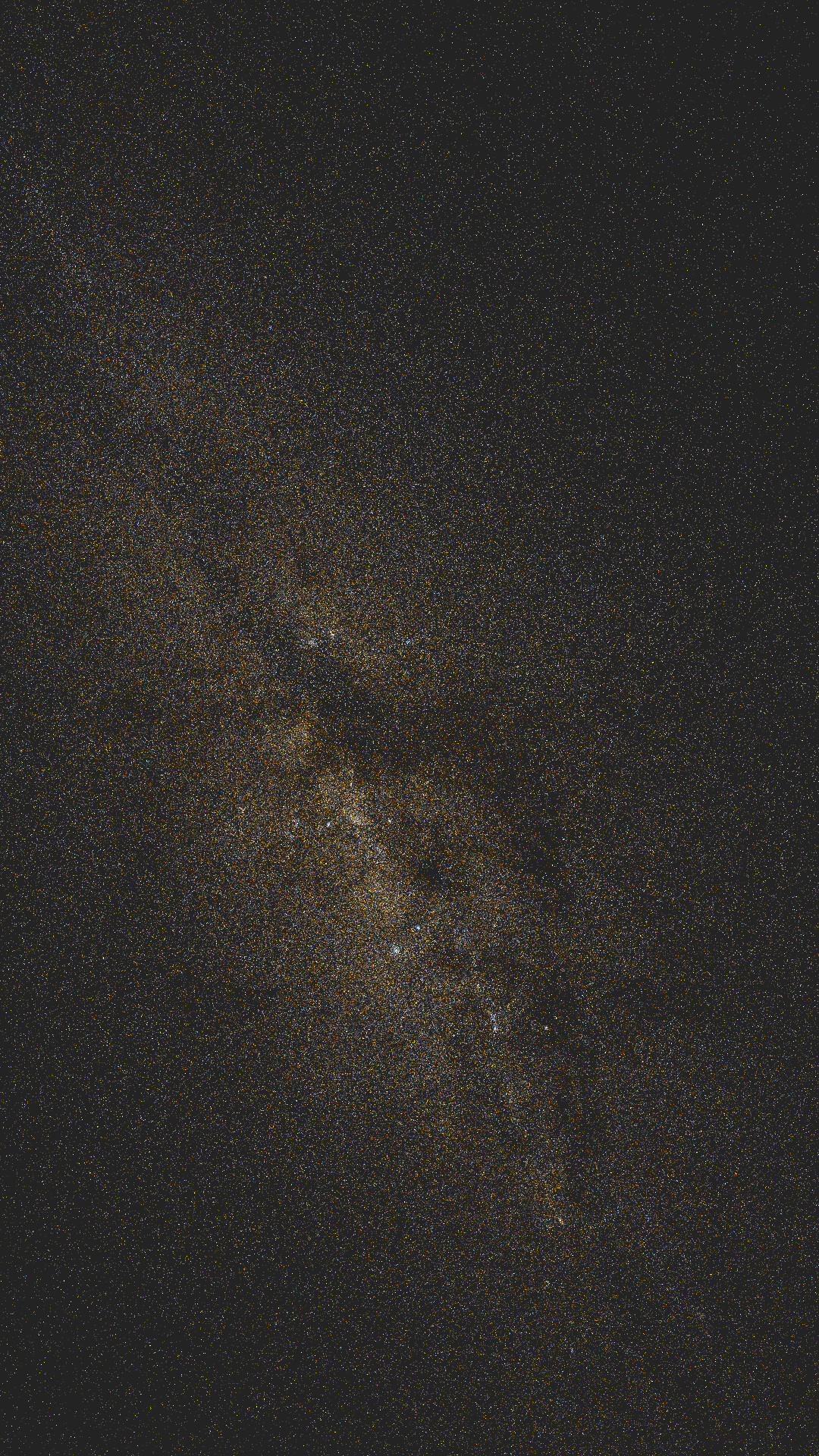
This is still catalog rendering, not a camera raw simulation. It explains how stars are distributed across the sky, how light pollution changes visibility, and how the display pipeline delivers the result to a screen. It does not simulate every optical defect of a real lens, nor does it aim for photometric-grade precision.

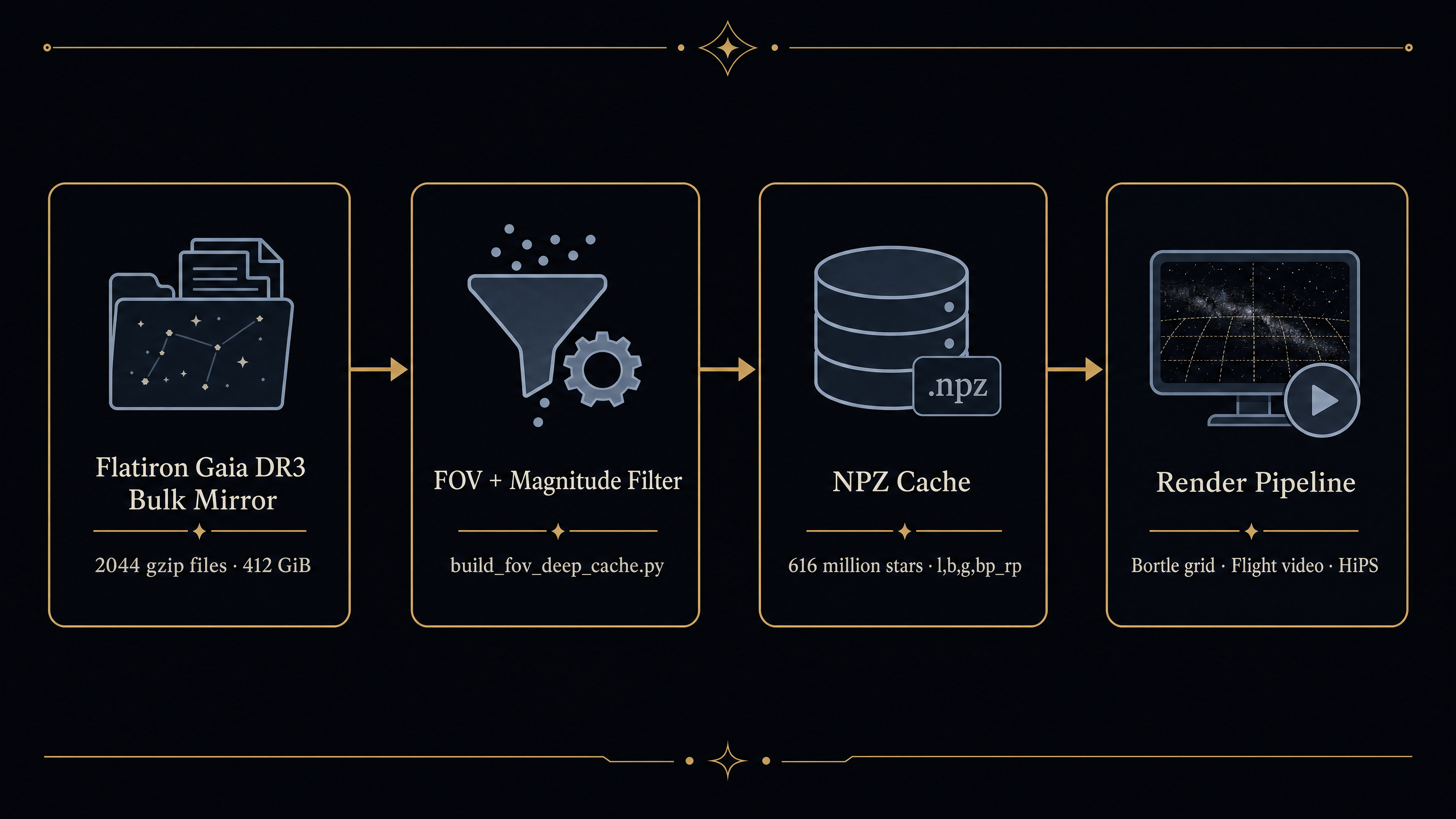
Gaia saturates or misses the brightest stars. Bright stars around G≲6 need to be supplemented with the Yale Bright Star Catalog BSC5. The current main cache adds a small number of BSC5 bright stars to the 616-million-star deep Gaia catalog, avoiding the absence of visual anchors such as Vega, Antares, and Altair.

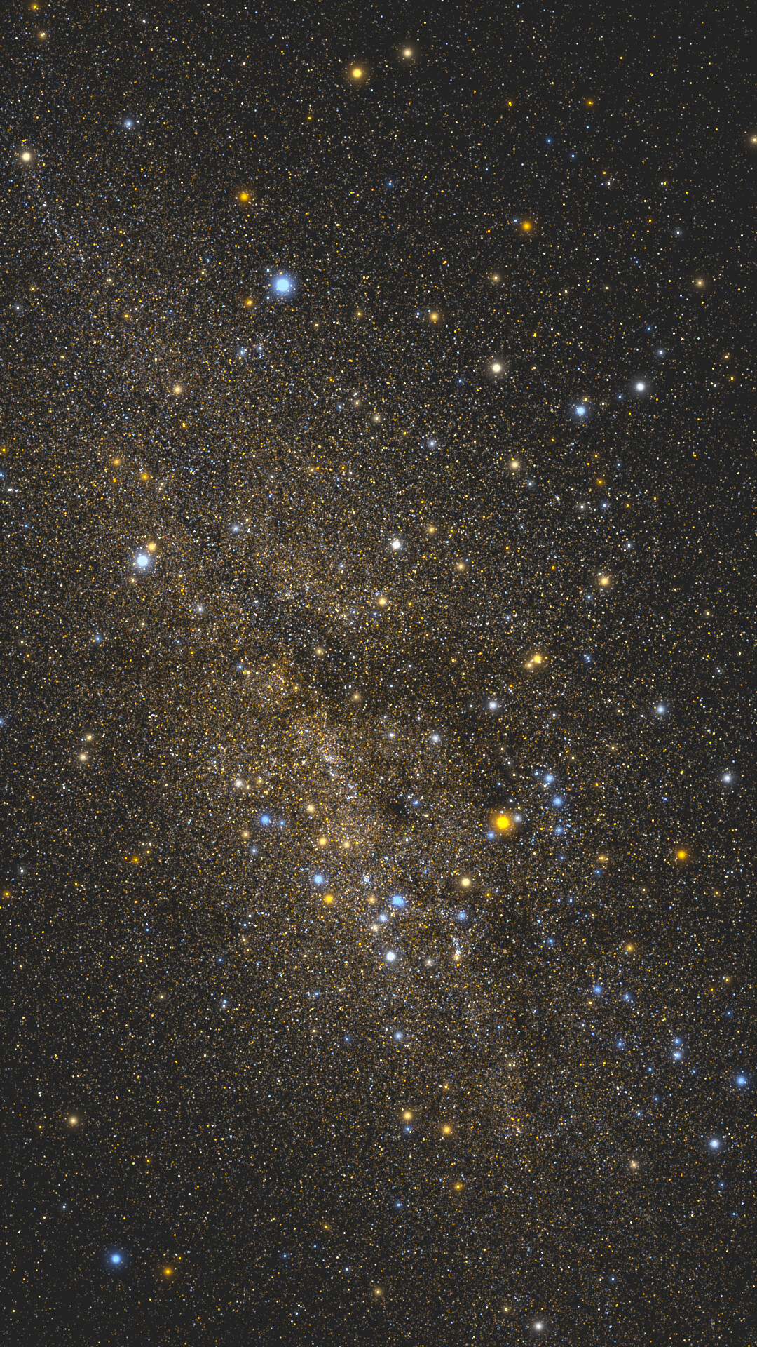
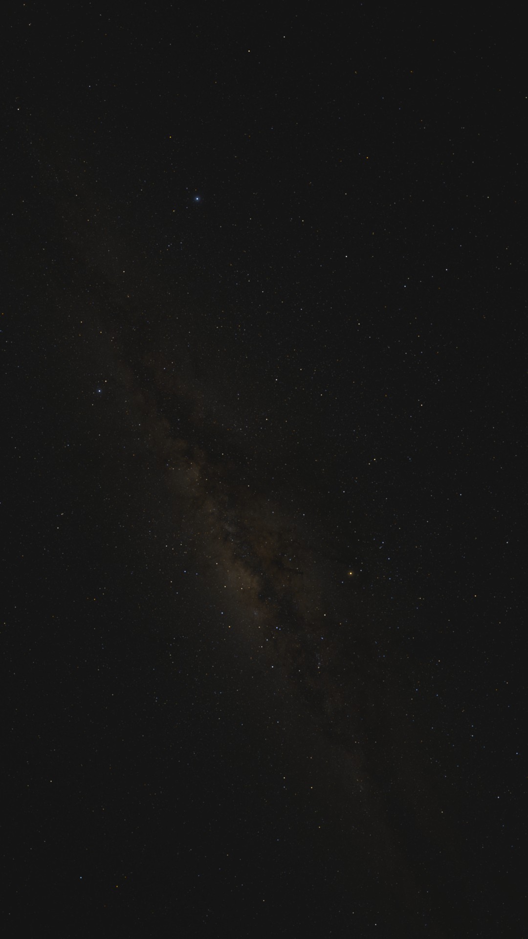
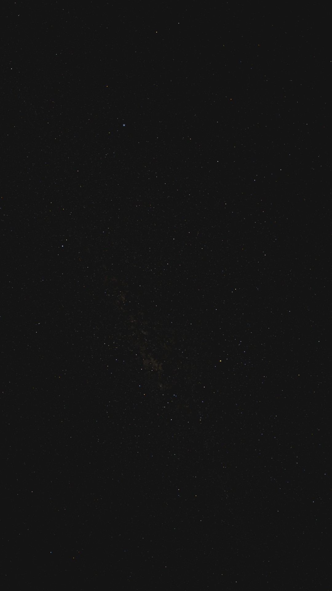
Gaia is a stellar catalog and does not include nebulae. The dark lanes in the image come from a reduction in visible stars. Nebulae themselves are not painted in separately. If a region has prominent red Hα emission or blue reflection nebulosity in real astronomical photographs, this project does not invent it.

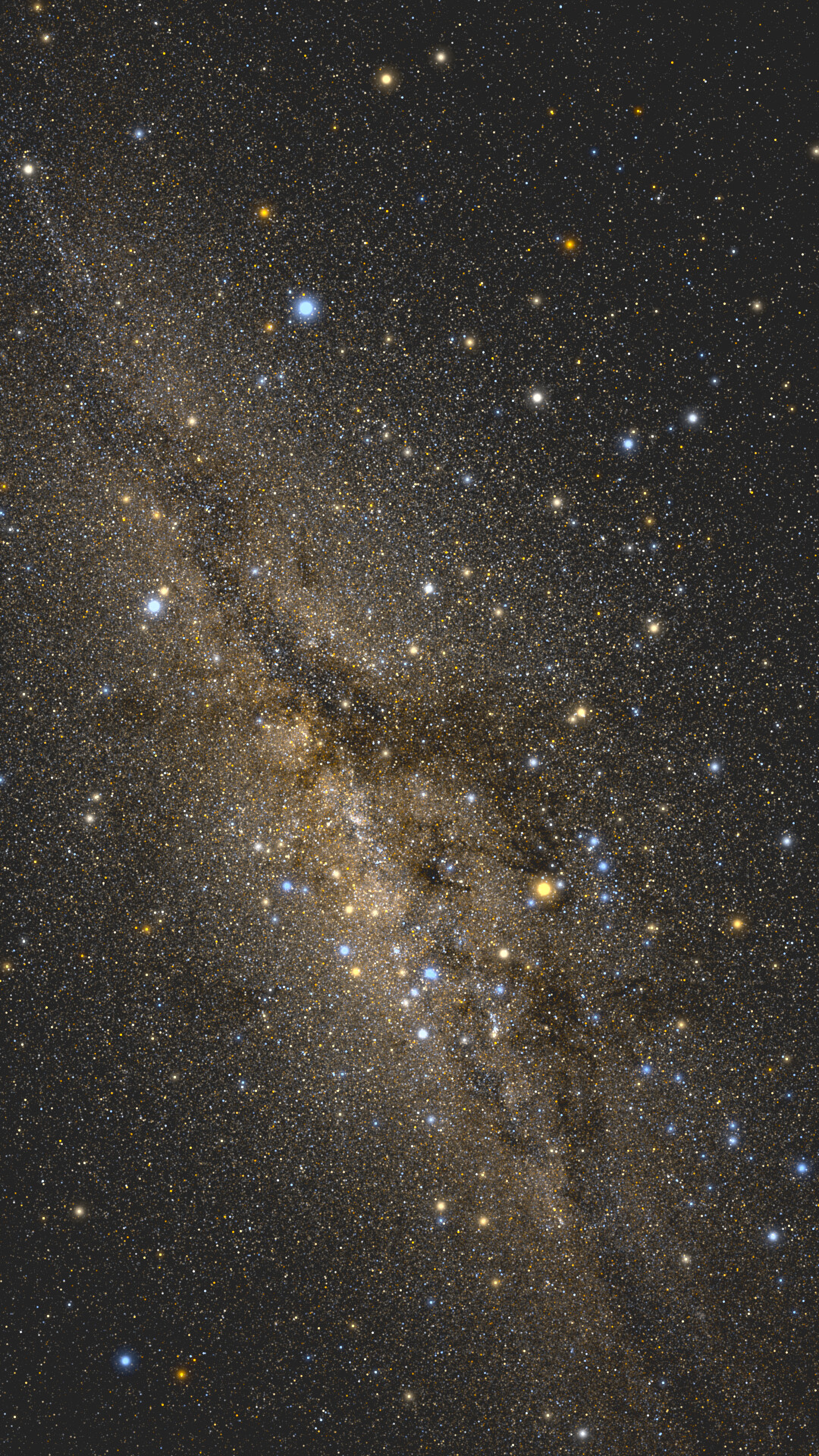
Gaia parallax is reliable only within a limited distance around the Sun. Its scale is roughly the local data sphere within a few thousand light-years. Flight videos can show constellations falling apart and nearby star fields being reprojected, but they cannot generate a true top-down view of the Milky Way. Humanity still has no such photograph.

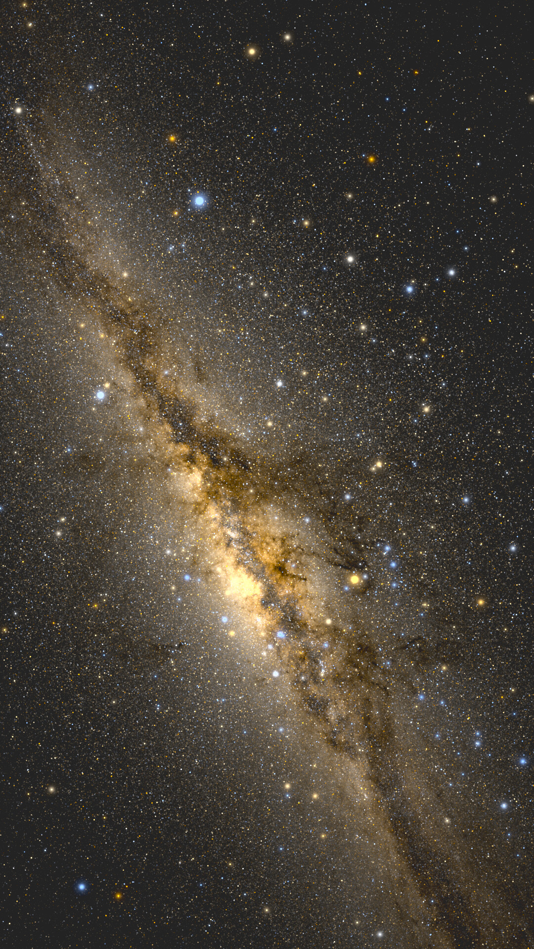
This is not an attempt to reverse long-exposure camera images into naked-eye vision. Long exposure, stacking, gradient removal, local curves, and color enhancement produce a different visual language. This project has a narrower goal: starting from Gaia stars, under clearly labeled display rules, to generate a traceable, reproducible, parameter-adjustable image of the night sky.

For full implementation details, docs/rfc.md in the repository is the complete design document, and docs/working.md records each round of parameter tuning and troubleshooting.